Beyond Uniformity: Modelling Real-World Variances with Modifiers

We simulate ideal devices, but we build real ones. The new ‘Modifiers’ feature in SunSolve Power allows you to model non-uniform electrical conditions (from manufacturing variance to partial shading) without re-running your ray trace.

In the lab, we strive for uniformity. In the field (and often on the production line), reality is defined by variance.

If you want to understand how your modules are going to perform for your customers, you need to consider the effects of real-world variance in your simulations. Shunt resistance varies across a batch of cells, series resistance can shift from wafer to wafer, and degradation after extended damp heat exposure is rarely uniform.

Until now, modelling these localized effects in SunSolve required complex workarounds. With the release of Modifiers, we have introduced a dedicated workflow to adjust equivalent-circuit parameters (J_L, J₀, R_s, R_sh) on a per-cell basis.

Whether you are a process engineer, a reliability specialist, or anyone exploring how to design better cells and modules, Modifiers give you the controls to quantify how sensitive your design is to real-world non-uniformities.

What are Modifiers?

Modifiers allow you to apply fractional (multiplicative) adjustments to the electrical parameters of specific cells or sub-circuits within a module. Previously, the closest approach in SunSolve involved tedious workarounds with localised illumination or manual post-processing. With Modifiers, you simply define multipliers. For example:

• 0.5 applied to R_sh: Halves the shunt resistance to simulate a micro-crack or localised defect.
• 0.2 applied to J_L: Reduces light-generated current to 20% to simulate heavy soiling or structural shading.
• 1.1 applied to R_s: Increases series resistance by 10% to model contact degradation or paste variations.

These modifiers can be targeted precisely : applied to a single cell (X, Y), an entire row, a column, the whole module, or even a specific sub-cell circuit within a tandem device.

Three Engineering Use Cases

There are many ways you could use circuit modifiers. Here are just three examples to demonstrate the new capabilities.

1. Non-Uniform Degradation

Degradation in the field is rarely uniform. Different cells in a module may degrade through different mechanisms, and Modifiers let you represent this directly. For example, increased recombination in specific cells can be modelled by raising J₀, while regions affected by potential-induced degradation can be represented by reducing R_sh. By applying these adjustments to targeted cells, you can study how different degradation modes — alone or in combination — affect module output power, and determine how much non-uniformity your design can tolerate.

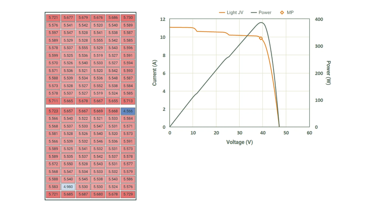
2. Bypass Diode Sizing & Behaviour

Validating bypass diode engagement is critical for shade-tolerant designs. Instead of setting up complex optical shading objects, you can simply apply a J_L modifier (e.g., 0.8 or 0.5) to a specific group of cells. This creates an intentional current mismatch, allowing you to trace the IV curve and verify exactly when the diode activates to protect the string.

3. Manufacturing Tolerances (Binning)

Production batches rarely have identical J₀ or R_s. Modifiers allow you to represent these batch-to-batch variations rapidly. You can simulate a “worst-case” scenario where specific cells in a module have higher recombination (J₀) or resistance, helping you establish robust binning criteria that account for real-world mismatch losses.

The Workflow Advantage: Iterate Without Re-Tracing

Beyond the engineering use cases above, there is an important workflow benefit: speed.

Modifiers are applied post-optical solve. Because they affect only the equivalent circuit parameters, you do not need to re-run the computationally expensive ray tracing engine.

• Run the optical solve once.
• Apply a modifier (e.g., shade a cell).
• Re-run the electrical solver instantly.

This allows for rapid iteration. You can test ten different shading scenarios or defect severities in the time it usually takes to configure one simulation.

The Takeaway

High-efficiency modules are increasingly sensitive to mismatch. The assumption of the “perfect wafer” is no longer sufficient for understanding reliability or yield.

With Modifiers, SunSolve Power provides the controls to model the device you are actually building, imperfections and all.

Read the full technical documentation on Modifiers here: docs.sunsolve.com